Chapter 5
How technology and science can support a sustainable way of living
Low energy collection was shown and discussed in chapters 1 and 2. They
were based on well known technology and science. Also mentioned was the
importance of architectural planning and designing to capture solar
energy. In this chapter, I tried to find how technology can contribute
to and support a sustainable way of living. It comes mainly from
architecture and environmental engineering where I have been involved,
and it obviously needs a lot of support from other areas of technology
and science.
First, it is mentioned how levels of each heterogeneous factor - noise,
thermal conditions and light - in the indoor environment can be
calculated. It is evident that they are key factors to guide us to a
sustainable way of living. They are not necessarily rigorous solutions
but practical enough to be used.
We have a variety of ways to take measurements, such as sound pressure,
light value, temperature, but they are just physical information. We
have to assess our environment with them after they simulate our
sensory systems.
Our living environment is composed of heterogeneous factors, such as
noise, thermal conditions, and light environment. They have their
specific subjective scales but we need combined evaluation to plan and
design a house. The theory of quantification was applied, introducing
an uncomfortableness scale to be common among them and for each factor
to be added linearly to be a combined total. It is actually the first
approximation for the purpose, but useful to compare and discuss each
factor in the room on the same basis.
They must be also balanced against strong economical forces where the
only motive is profit. Our society is so distorted from a healthy form.
Our sensory systems are dynamic and should be noted in the transient
form for fluctuating inputs. Technological and scientific measurements
must be evaluated through our perception. Studies of subjective
responses are very relevant.
An example of combining factors will be given as well.
Architectural
environmental planning
A) Flow chart for architectural planning and designing
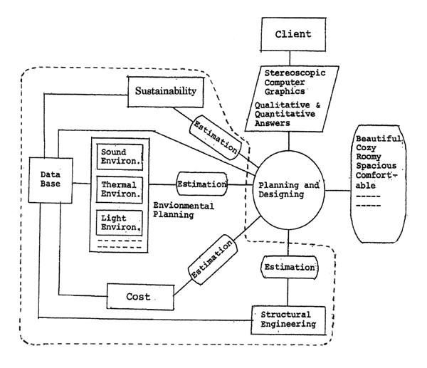
A computer program whose flow chart is given in Fig. 1 assists
architects. The computer program is expected to feed back in real time
with the output for each item enclosed with a dotted line. He can
concentrate on house planning, designing and talking with his client
through a three dimensional view.
Fig.1 Flow chart for house designing
The estimation function for sustainability is not given yet, but its
total score can be obtained with the total of positive and negative
points given by the comparison with the sustainable level at the
experimental house at Kaiwaka.
Noise level, thermal conditions and light for indoor environmental
planning can be calculated physically. The indoor environment can be
predicted as mentioned later. Combined rating for a living environment
is also given.
Cost effectiveness and the estimates for structural engineering are
well established.
The data base to support all these functions must be well established
to be directly usable by the architect.
The data base must be given for a general view and not only for a
specific item. Namely, not only its particular physical data for each
material, but any other physical data when it is used for construction,
such as the energy consumption during production, the amount of
hazardous waste, durability and so on. They should be filed and applied
to architectural design.
B) Physical field calculation for three architectural environmental
factors in their simulated specific scales
Practical calculations are given for three environmental factors. They
are not rigorous ones but practical enough to be used for planning and
designing a house.
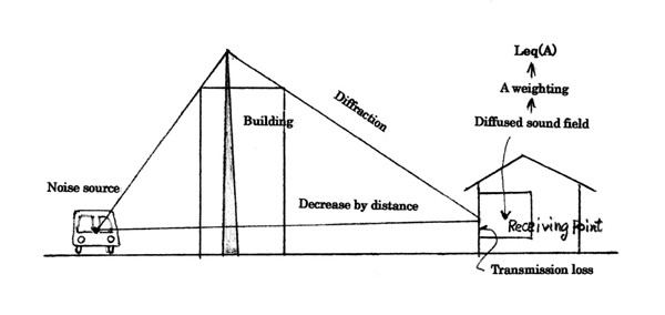
B-1) Sound level (Leq (A))
A noise travels to the receiving point in a house as shown in Fig.2.
Fig.2 Noise reduction
from a noise source to the receiving point in a house
B-1-1) Decrease by distance
When a point source of power W (watt) is located at a distance r (m)
from a receiving point, the intensity I (watt/m2)
at the receiving
point is given as follows, because the source power is distributed over
a sphere surface of 4πr2
I = W/4πr2
The level L (dB) is given by the definition,
L = PWL-11-20log10r (dB)
where PWL=10log10W/I0
(dB) and I0 is 10-12watt/m2
that is the international standard. 10log104π
is approximated to 11.
When levels at r1 (m) and r2 (m)
are L1 (dB) and L2 (dB),
respectively,
L1 =
L2-20log10r2/r1
(dB).
If r2 is double r1, L2
decreases by 6 (dB).
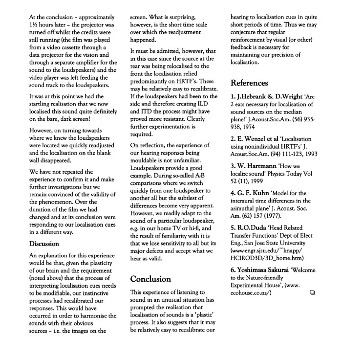
B-1-2) Decrease by diffraction
If a semi-infinite thin barrier is placed between a sound source and a
receiving point, the sound level can be expected to decrease. This
insertion loss is given on the vertical axis (dB) in Fig. 3. The
horizontal axis shows Fresnel’s number
N=2δ/λ, where
δ shows the path difference from the direct distance and
λ
a wavelength. If the path difference over the barrier is larger, the
noise level decreases and it is more effective for higher frequencies.
When a barrier has thickness, it is replaced with an equivalent thin
barrier as in Fig.1 to get the insertion loss. It gives more loss at
low frequency, though. It is discussed in chapter 6.
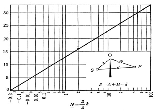
Fig. 3 Insertion loss by a thin semi-infinite screen (by Z.Maekawa)
When a noise of L1 (dB) impinges an outside wall
surface and comes in
through a wall which is composed of a few different materials and whose
average transmission coefficient is τ, inside level L2
(dB) is,
L2 = L1-TL-10log10A/4S
(dB),
where TL is transmission loss of the wall, A is the absorption of the
room and S is the area of the wall. τ is given by Σsiτi/S
and TL is 10log101/τ.
Suppose the wall of 20m2 includes an opening of
0.5m2, a glass window
of 4.5m2 and a concrete wall of 15m2,
whose transmission loss is 0, 20
and 50dB, respectively, the average transmission coefficient τ
is
τ =
(1x0.5+0.01x4.5+0.00001x15)/20 = (0.5+0.045+0.00015)/20 = 0.5/20
The sound transmission through the wall is dominated by the opening. If
it is shut, τ is 0.05/20. The highest transmission part
dominates
it.
B-1-4) Sound field in an enclosure
If a sound field in an enclosure is diffusive, the energy which falls
over its surface is EC/4 per a square meter where E (Joule/m3)
is
energy density and C (m/sec) is sound velocity. The factor 1/4 can be
understood as being caused by the random incidence on the surface.
The diffused sound field E is produced by the energy from the first
reflection of a given sound source of power W in the enclosure,
W(1-α) =
ECSα/4,
where S (m2) is the surface of the enclosure and
α is the
average absorption coefficient of the surface. Energy density at a
receiving point is given by the direct sound and the diffused sound,
E = W/4πr2C+4W(1-α)/CSα
If all the given energy turns out to be diffusive,
E = 4W/CSα
When a sound level L1 (dB) is at a surface of
absorption coefficientα1 and L2
(dB) at α2,
L2
= L1-10log10α2/α1
(dB)
When the absorption coefficient changes fromα1
= 0.05 to α2
= 0.30, L2 (dB) decreases by 8dB. Whenα1
= 0.30 and it is changed
toα2=0.5, L2
(dB) decreases by 2dB. The former treatment is worth
doing, but the latter is not.
B-1-5) General steps to take for noise control
First is to suppress the noise at source. Second is to reduce noise
through by distance. Third is by placing buildings in between. Forth is
by the sound insulation at the wall of the room. Don’t expect
much from absorption in the room.
B-1-6-1) Weighting for the loudness of a noise
A noise has a broad spectrum band. As previously mentioned, sound paths
are frequency dependent. First, physical calculation must be done for
each band level until it reaches a receiving point.
To estimate the loudness of a noise and make it to be comparable with
the loudness of another noise, it must be weighted to our hearing
system. Fig. 4 shows “A” weighting curve with a few
other
weighting curves. It is weighed for each band level of the noise in dB
to give each band weighting and added up to have dB (A) for the noise.
“A” weighting curve is obtained from the loudness
comparison of pure tones. It should be done for a broad band noise
which includes non-linear responses. It is discussed in the chapter 6.
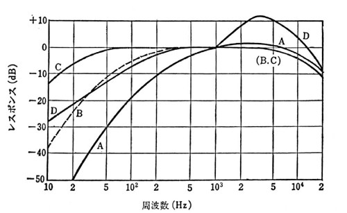
Fig.4 Weighting curves for a noise
B-1-6-2) Evaluation of fluctuating noises with Leq (A)
In order to evaluate fluctuating noise into one figure, the time
average of “A” weighted values is introduced to
call Leq
(A). Namely,
Leq
(A) = 10log10(1/N∑10Li /10)
(dB (A) )
Li (dB (A)) is a noise level sampled for a certain time interval. N is
the total number of samples for the time interval. High levels in the
duration are well weighed.
B-2) Thermal conditions in SET*
Our thermal sensation is changed not only by air temperature, but also
by humidity, radiation, air movement and how thick the clothes we wear,
namely a “Clo” value. SET* is the estimation unit
to
include their effects.
B-2-1) Thermal equation
Thermal transfer must be solved in the transient form and it needs to
be estimated with the inclusion of heat capacity.
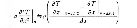
It occurs in three dimensions, but it is sufficiently approximated by
solving it in one dimensional when it is used for boundaries of a
house, e.g. a wall, a ceiling and a floor. The thermal transfer
equation is given by,

where T (℃) is temperature and depends on two variables time t (sec)
and place x (m). Thermal diffusivity a (m2/h) is
expressed as,

where λ(kcal/mh℃) is the heat transfer coefficient, c
(kcal/kg℃) is the specific heat and ρ(kg/m2)
is density. The
initial and boundary conditions are needed to solve the equation.
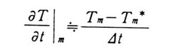
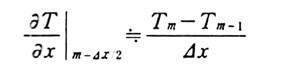
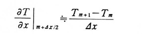
B-2-2) Finite difference equation for thermal transfer (This section
referred to Dr. Udagawa’s book written in Japanese)
A wall has outside air temperature Ta(0) and inside air temperature
Ta(M), when the wall is equally divided into M layers with the width
Δx, temperature at m is expressed as Tm shown in Fig.5. Each
point is named 0, 1, 2, m, . . ., M from the left surface to the right.
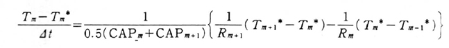
The finite difference equation at m is obtained,
Fig.5 Finite difference expression for thermal calculation of a wall
where
and
where Tm* is the temperature at ( t-Δt ), namely the one
beforeΔt.
Finally,
This form is called the forward-difference method. Tm at time t of
point m is calculated by the known temperatures Tm* before Δt.
However, it needs a certain condition to be satisfied for calculation.
The following backward-difference method is applicable at the
condition; it needs to be solved with linear equations for the
temperature at t of each point. It is given by,
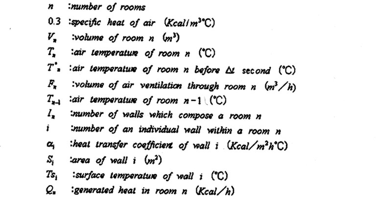
B-2-3) Equation of heat balance
The heat stored in a room as the temperature changes from Tn to Tn*
should balance with the total heat gain by the air movement to the
adjacent rooms, through the boundaries and generated heat in the room.
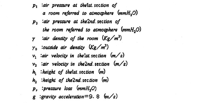
B-2-4) Equation of air movement (Bernoulli’ formula)
Temperature change in the room changes air movement. It is given by the
Bernoulli’ formula as bellow,

B-2-5) Linking two equations
Linking two equations for the heat balance and air movement for a
central point of a room is done and it was done in the same way for the
whole system as shown in Fig.6. For thermal transfer, the backward
difference method was applied and the linear equation was solved by
iteration.
Calculation was done for a point in a room and temperature distribution
in the room must be considered afterwards.
To get combined rating for thermal conditions the scale of SET* is
introduced. It is expressed with the effects of air temperature,
humidity, air movement and “Clo” value.
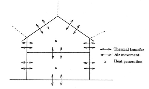
Fig.6 Linking the two equations
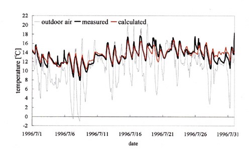
B-2-6) Comparison of measured and calculated temperature changes
Calculated results are compared with measured results at the
experimental house in Fig. 7 and 8. They were done by Hirotaka Azumi
(Hirotaka Azumi Environ. & Build. Research. Email address:
hirotaka_azumi@nifty.com ). He was then my student.
This computer program simulates the measured results well, especially
their changes and is of practical use.
Fig.7 Measured and
calculated temperature changes in the bed room, in winter of 1996.
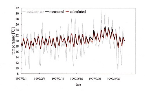
Fig.8 Measured and calculated temperature changes in the bed room, in
summer of 1997
B-3) Light environment in lux (This section refers to Dr.
K.Matsuura’s book written in Japanese)
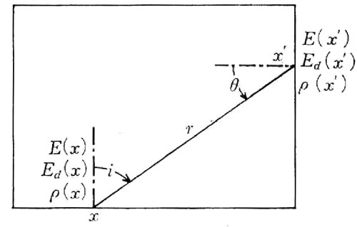
B-3-1) Integral equation for indirect illuminance
Indirect illuminance occurs with the inter-reflection between the
surrounding boundaries, whose surfaces are uniform diffusive namely
they follow the Lambert cosine law. A room is composed of the diffusive
reflecting surfaces as shown in Fig.9.
Fig.9 Mutual reflection
of indirect illuminance on the room surface
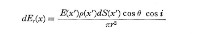
When the total illuminance is E(x) (lx), the direct illuminance Ed(x)
(lx), the indirect illuminance Er(x) (lx), the
reflectance ρ(x) and
a surface segment dS(x) at a receiving point x, the received
illuminance at x from a surface element dS(x’) at
x’ is
given,
The indirect illuminance at x, Er(x) is given
with the integration of the whole room surface S (m2)
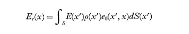
The total illuminance E(x), which is Ed(x) + Er(x),
is given with the Fredholme Integration Equation of the second kind as

The integral equation can be solved for E(x) with the linear equations.
B-3-2) Equivalent reflectance method
When the whole inside surface is treated to have a uniform indirect
illuminance, the following practical calculation through (1) to (4) is
possible.
(1) After a direct luminous flux Fd (lm) gives
the direct illuminance,
it is reflected and creates the indirect illuminance, Er
(lx) The first
reflected luminous flux Fr (lm) is the one
absorbed at the
mutual-reflection. When the average reflectance of the inside surface
S(m2), is ρm, Fr
is equal to the absorption Er (1-ρm)S.
Fr is
approximated Fdρm.
Then, Er is given by,

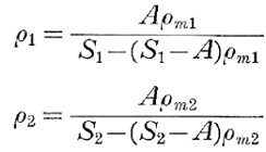
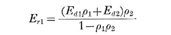
(2) When relatively large surfaces 1 and 2 are facing in parallel with
each other, the direct illuminance of each surface is Ed1
and Ed2, the
indirect illuminance Er1 and Er2
and reflectance ρm1
and ρm2 , respectively,

Then, the indirect illuminance on the surface 1, Er1
is given by
(3) Equivalent reflectance
When there is a cavity as shown, having luminous flux impinging on the
aperture Fi
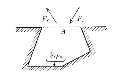
Fig.10 Equivalent reflectance at the mouse of a cavity
and reflected one there Fr, an equivalent
reflectance of the
aperture ρe is given by Fr/Fi.
When the internal indirect
illuminance of the aperture is Era and the
indirect illuminance of the
inside surface S of the cavity is Ers, Era
is given by,
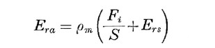
where ρm is the average
reflectance of the inside surface.
Once reflected luminous flux in the cavity, Fiρm
is absorbed
producing the indirect illuminance Era and Ers,
namely

where A is the aperture area.
Era is obtained by Fr/A,
then, ρe is given by

(4) When a room is cut at a desk level for instance, the I-I and II-II
apertures are obtained as shown, and each has the equivalent
reflectance ρ1 and ρ2
,
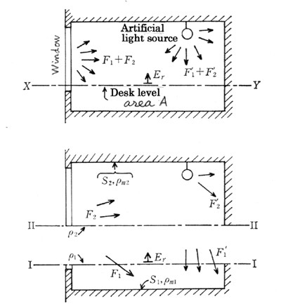
Fig.11 Application of the equivalent reflectance method for illuminance
Er at desk level
where S1 is the room surface area above the
section level and S2 is
the one below the level, ρm1 , ρm2
are the average
reflectance for S1 and S2,
respectively. A is the area of the section
at desk level.
When two parallel planes of equivalent reflectance are facing with each
other, the indirect illuminance on the S1, Er
is given using the result
in (2) by,

where F1 is the direct luminous flux from the
windows and lights to the I-I level and F2 is
the one to the II-II level.
Each field calculation in this section B) is done numerically. Each
boundary must be well divided for the numerical calculation of three
factors to be used consistently.
C) Theory of Quantification II by Hayashi (Computer program is given on
the Statistics Package for Social Sciences.)
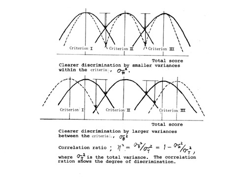
Fig.12 Correlation
ratioη2 with variances within a criterion or between criteria
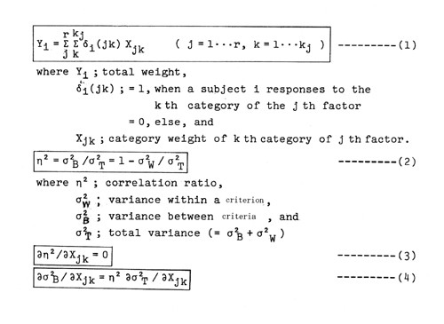
This is one of the quantification theories by Hayashi, which is called
II.
When
there are criteria in a multi-variable field which need to be clearly
distinguished , correlation ratio η2 is
introduced as a measure to show
its degree of distinction. When the variance of each criterion,
σW2, is
smaller, the valley in between becomes deeper, namely each criterion is
distinguished more clearly. When the distance between criteria,
σB2 is
larger, it becomes deeper too. They are related with the variances,
σT2
=σW2 +σB2.
The correlation ratio is standardized by the total variance.
It
is very useful when criteria and their factors are expressed with
categories. Namely, they are qualitative but they become quantitative
by the application of the theory.
D) Combined rating of indoor environments
Combined rating of three environmental factors in a room for steady
state using the Theory of Quantification II is given.
When
each heterogeneous factor is expressed with its specific subjective
scale, it is impossible to compare with each other and combine them.
But when it is rated on uncomfortableness, namely stress, it becomes a
common scale for them as shown in Fig.13.
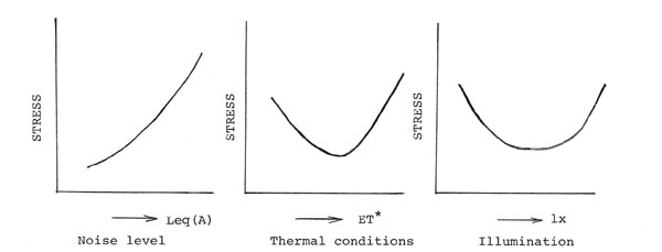
Fig.13 Introduction of a
common subjective scale for three heterogeneous environmental factors
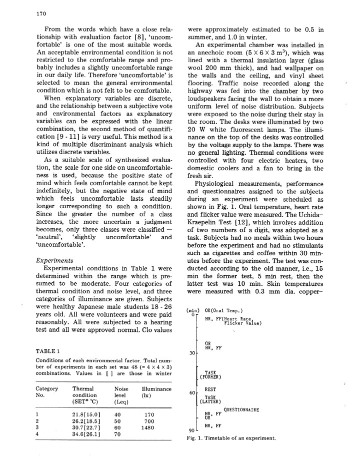
Trial
volunteers did simple addition work in the artificial climate chamber
whose noise level (LeqA), temperature (SET*) and light (Lx) were
changed. They were asked how they felt while they were working,
“Neutral”, “Slightly
uncomfortable”, or “uncomfortable”.
After the application of the Quantification Theory II, the category
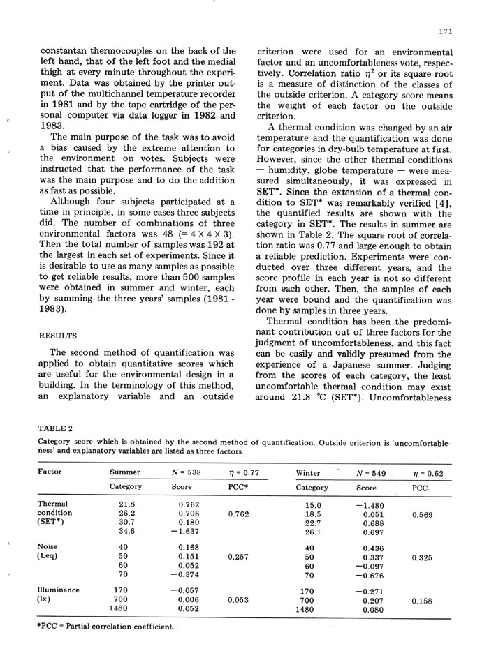
scores for each factor were obtained as in Table 1.
Table 1 Category scores
of noise level (LeqA), temperature (SET*) and light (Lx) to rate an
indoor environment
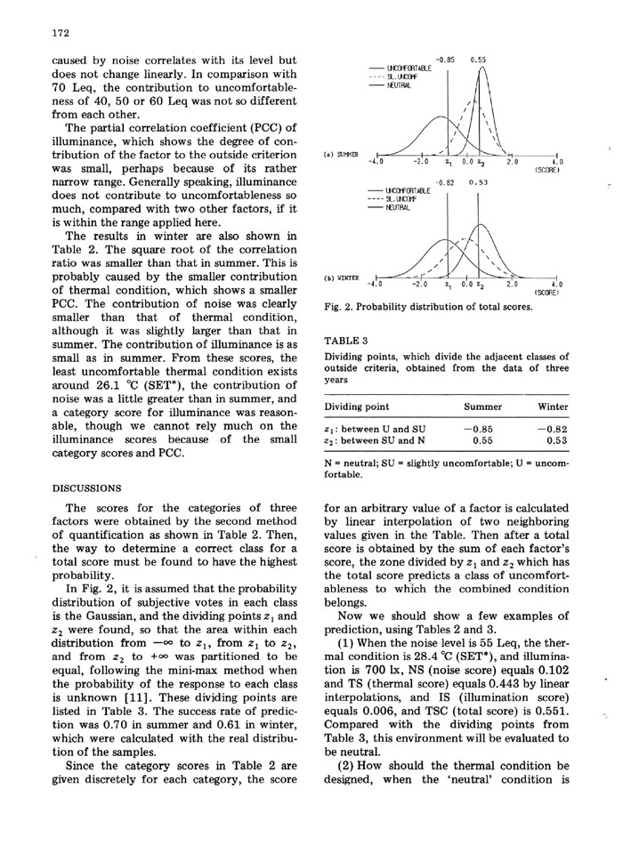
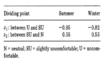
Now,
we have to find the dividing points to distinguish each criterion. It
was divided to have an equal area of response curve between two
dividing points following the mini-max method when the probability of
the response to each criterion is unknown. They are given in Table 2.
Table2 Dividing points
for each criterion
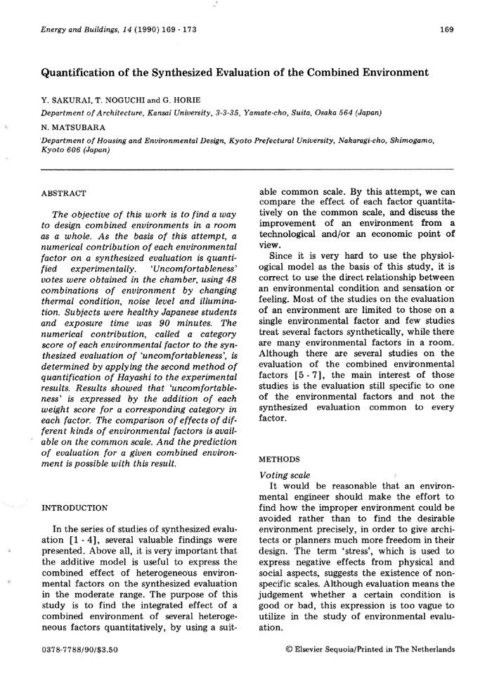
Reference: Y.
Sakurai, N. Matsubara : ”Quantification of the Synthesized
Evaluation
of the Combined Environment”, 14(1990),169-173, Energy and
Buildings
(Elsvier).
The next five pages are copied from the above reference
E) Combined rating of a living environment
Twenty-three factors were prepared for social survey of a living
environment to apply the Theory of Quantification II.
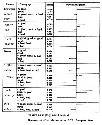
Table 3 Category scores
for combined rating of a living environment
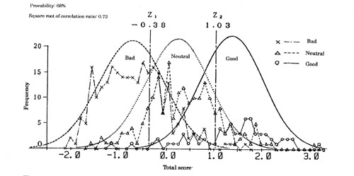
Fig.14 Dividing points for combined rating for a living environment
Most
of present residential areas in Japan are city environments and the
internal correlation between each factor in twenty-three was high. They
were reduced to eight factors to fulfill the application condition of
the theory, where each factor must be independent. Even with eight
factors the prediction was correct over 70% of the time when it was
tested on my students for several years. Category scores and the
dividing points are given in Table 3 and Fig.14, respectively.
Categories of a factor were collected to have higher correlation ratio.
Reference;
Y.
Sakurai et al: “Quantitative Environmental Planning Based on
the
Analysis Using the Theory of Quantification II”, Journal of
the Archi.
Inst. of Jpn, 387, p53-60 ( in Japanese ).
When this evaluation method is applied to our experimental house at
Kaiwaka,
| Shopping convenience |
Bad |
-0.251 |
| Winter sun |
Very good |
0.303 |
| Night lighting on the road |
Bad |
-0.113 |
| Noise |
Good |
0.241 |
| Traffic safety |
Good |
0.023 |
| Greens surroundings |
Very good |
0.216 |
| Public security |
Good |
0.382 |
| Child safety |
Neutral |
0.068 |
The
total score is 0.733. When it is estimated referring to the dividing
points in Fig.14, it is “Neutral”, though it is
very close to “Good”.
For instance if shopping convenience is improved, the rating changes to
“Good”. This result accords with my daily
impression.
The analysis is based on one’s satisfaction. It should be
categorized with more objective categories.
F) Theory of quantification I by Hayashi
It
is a methodology to find a numerical value for an outcome, which
changes with independent multi-variable factors and they are expressed
qualitatively in categories.
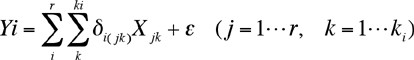
Yi is a given outcome of a subject i.
When a subject i responses to the k th category of the jth factor,
δi(jk) takes 1 and otherwise 0, Xjk
is a category score of the kth
category of the jth factor to be found, a given value Yi is
expressed,
where ε shows an error term.
Here,
we want to find Xjk which make error term
ε smallest using the least
squares method, namely, it is to make ε2 smallest. Now,
ε2 is partially
differentiated by Xjk and its result is made
zero. Finally, r x kj
linear equations are obtained and must be solved simultaneously.
F-1) A few applications of the theory of quantification I
A few examples where we applied the theory of quantification I are
shown in this section.
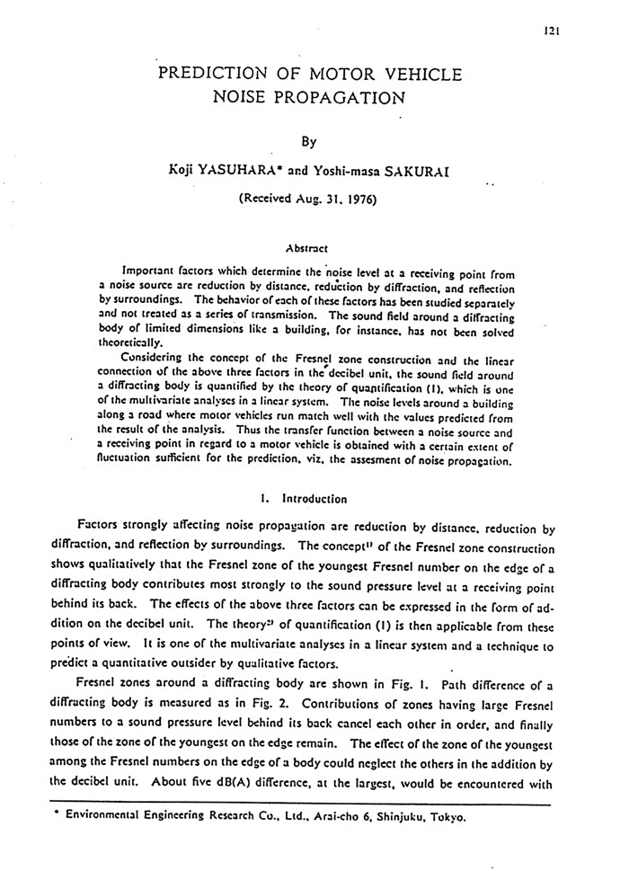
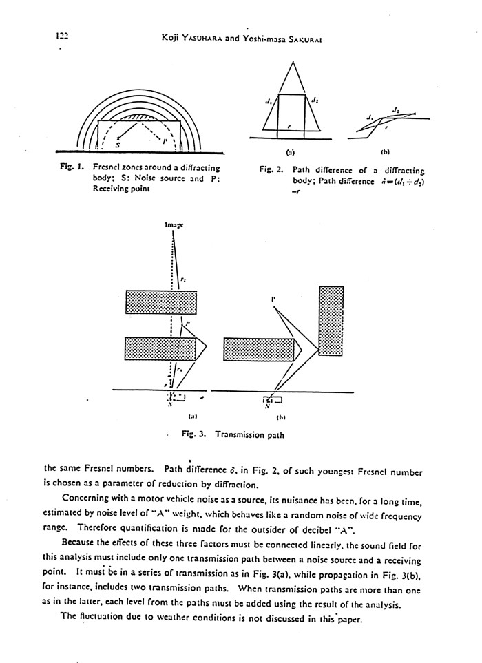
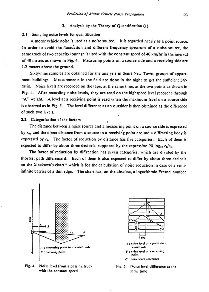
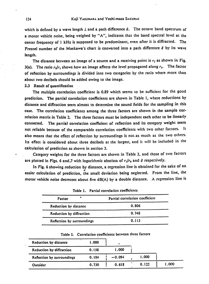
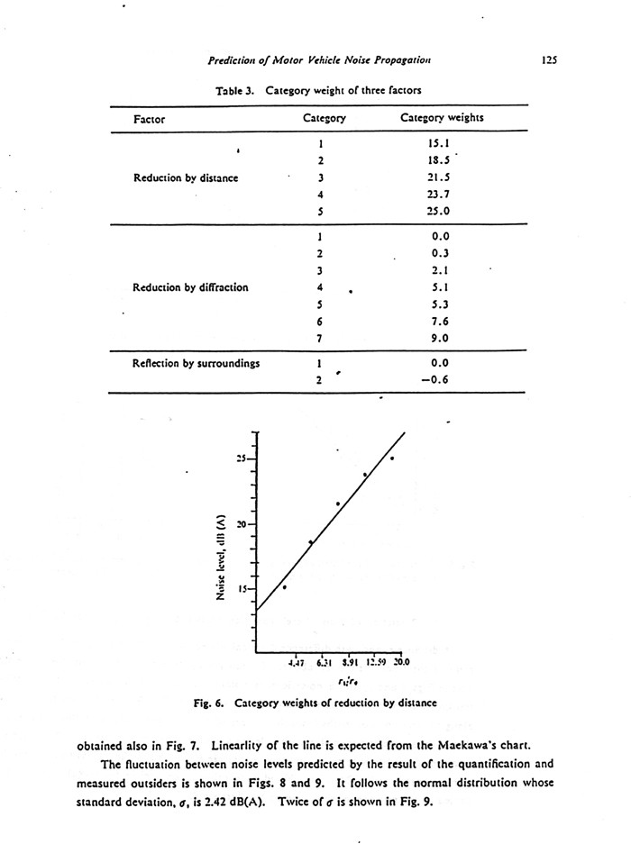
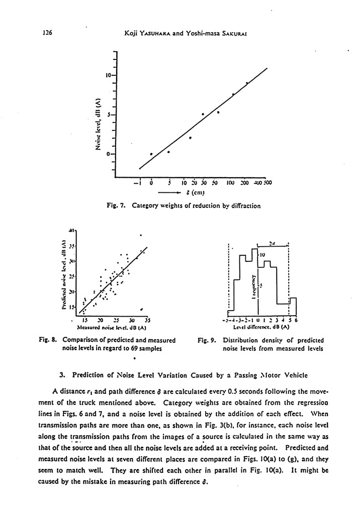
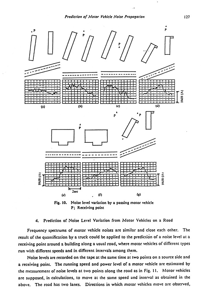
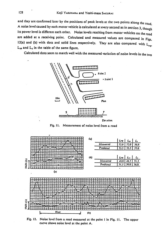
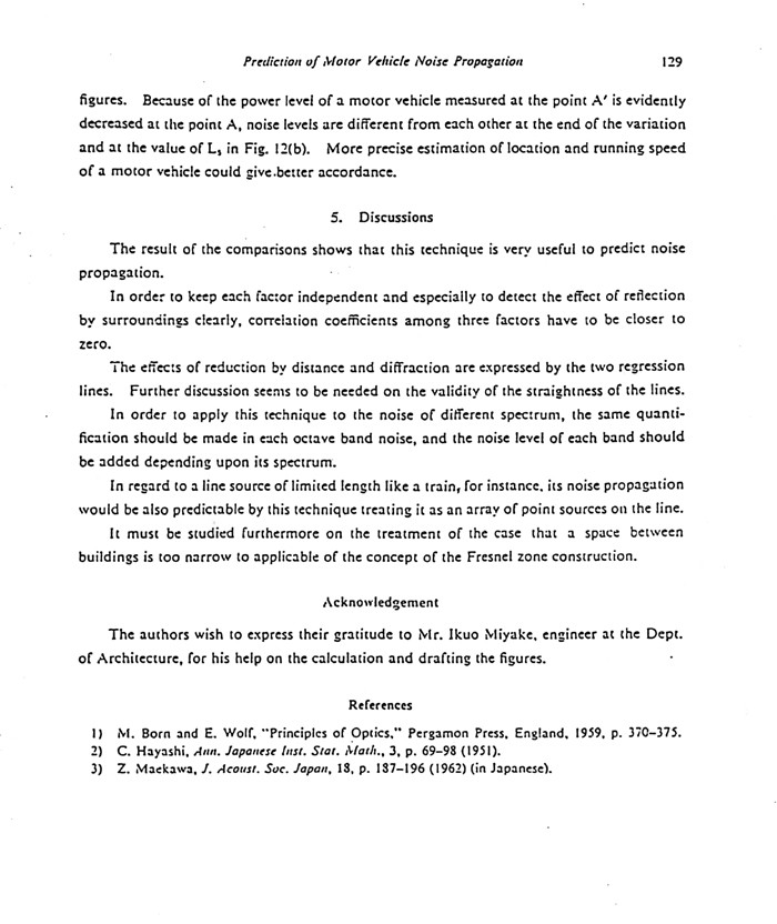
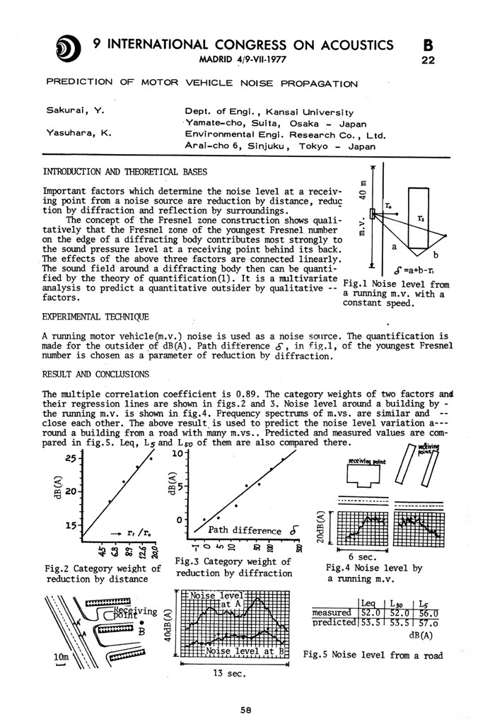
F-1-1) Prediction of motor vehicle noise propagation
The following paper was published on the Technology reports of Kansai
University March, 1977.
The next paper is a summary of the above paper given at the 9th
International Congress on Acoustics in Madrid, 1977.
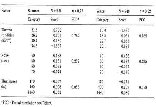
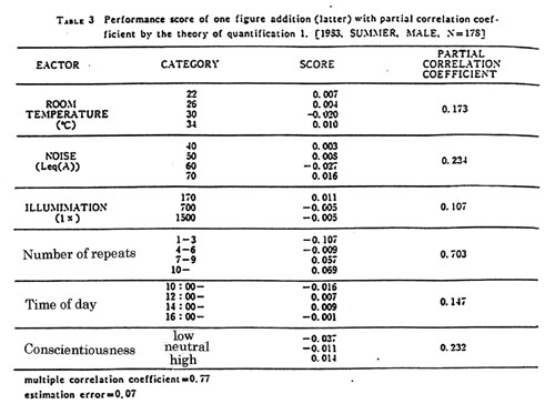
F-1-2) The effect of environmental factors on the performance test of
adding two single digit numbers
As
a performance test, Kraepelin test was given which is adding two single
digit numbers. To distinguish each volunteer’s ability a
performance
was divided by his/her average performance. The result of how
environmental factors affect the performance is shown in the next table
with the application of the theory of quantification I.
As
it is shown, the factor of how many times he/she took the test is
dominant. It is caused by the learning effect. Among environmental
factors, the noise environmental shows the largest partial correlation
coefficient, but they do not show much influence on the performance.
G) Suggested area of applications of the theory of quantification I and
II
Not
only our living environments, but also agricultural productivity,
various industrial systems etc are changed under multi-variable
factors. Even if their results are approximated by the linear addition
of each factor’s contribution, they are still useful to
precede further
discussion. Here are some suggested areas to apply the methodologies.
G-1) Applications of the theory of quantification I
(a)
Air convection in a room is not easily to solve on the equation,
because it behaves non-linearly. However, temperature distribution
there is layered in most cases. If layering is assumed, it may be
approximated with the theory of quantification I to have the
temperature difference from low to high in the room as the outcome and
to have dimensions, surface curvatures, shapes, furniture and so on as
factors. It needs experimental approach.
(b) Fruit growing
Possible
factors: orientation to the sun, soil quality, seed, area for a tree,
geographical situation (flat or slope), climate and so on.
(c) Vegetable growing: similar as (b)
(d) Crops growing: similar as (b)
G-2) Applications of the theory of quantification II
(a) Causes of cancer
Outcome: Suffered or not
Possible factors: genetics, diet, stress, daily routine, age, junk food
and so on.
H) Rating of fluctuating environmental factors
We must know how an environmental factor changes, and the sensory
systems respond to it. Referring to their relationship, we have to plan
or improve our living environments. For instance, the thermal change in
a room must be solved in the transient form other wise it is not
meaningful. The thermal sensation should include its changing nature.
For that, its linear response in the early stage the system must be
known and be appropriately applied to environmental planning.
H-1) Sound
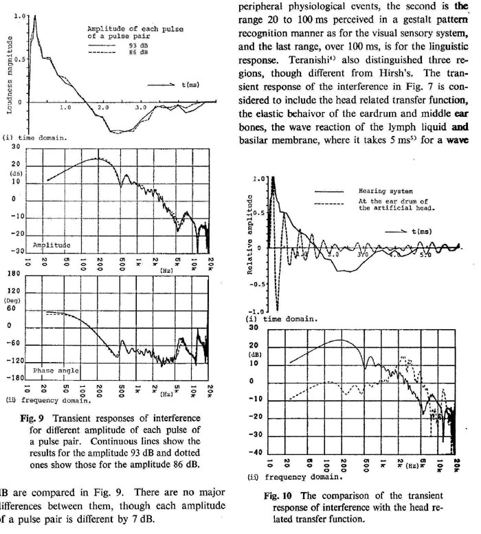
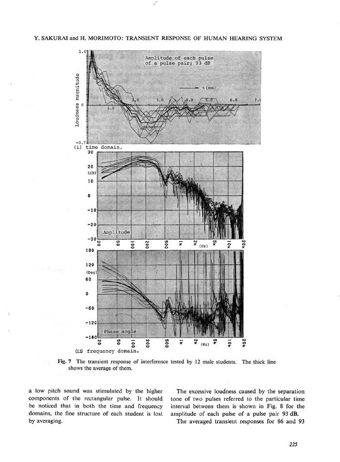
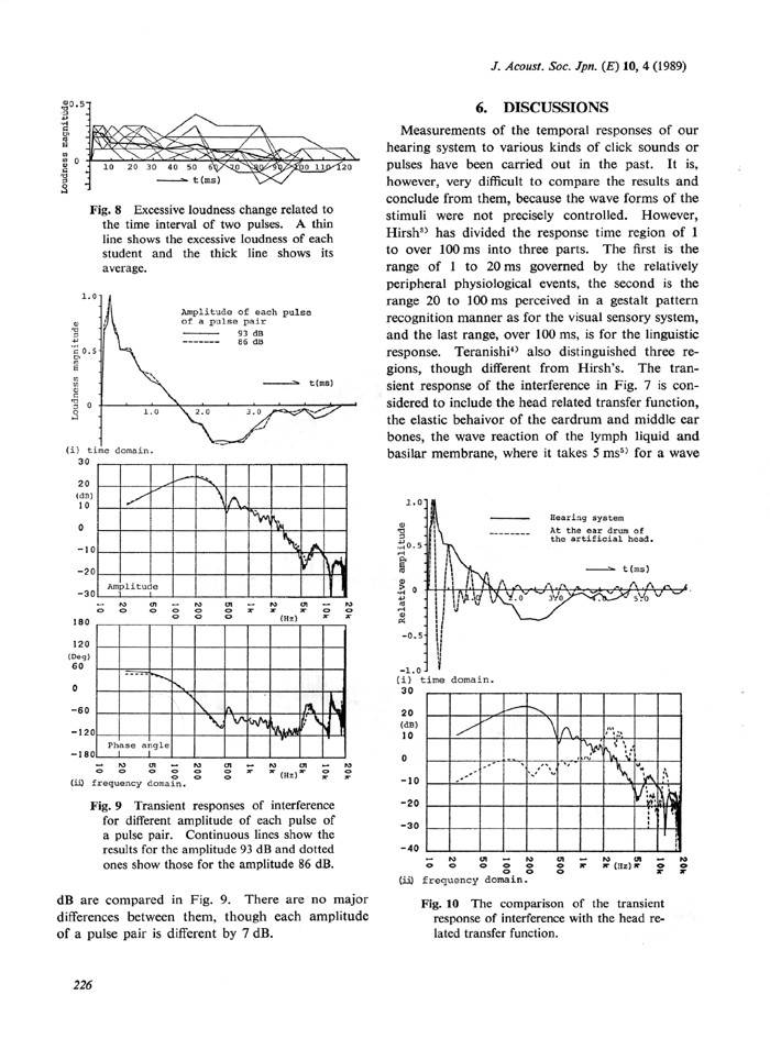
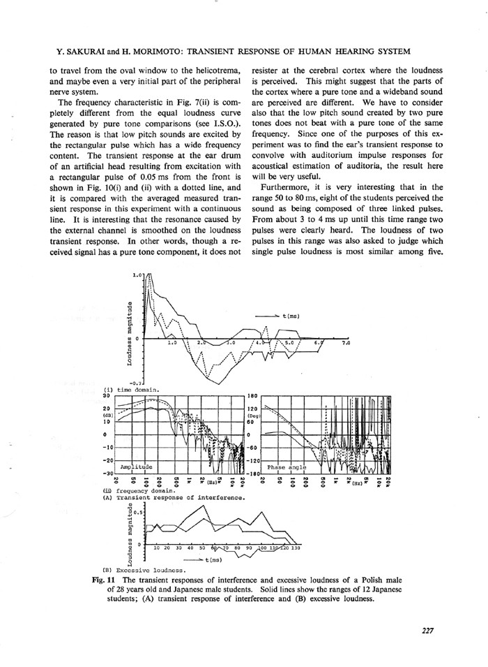
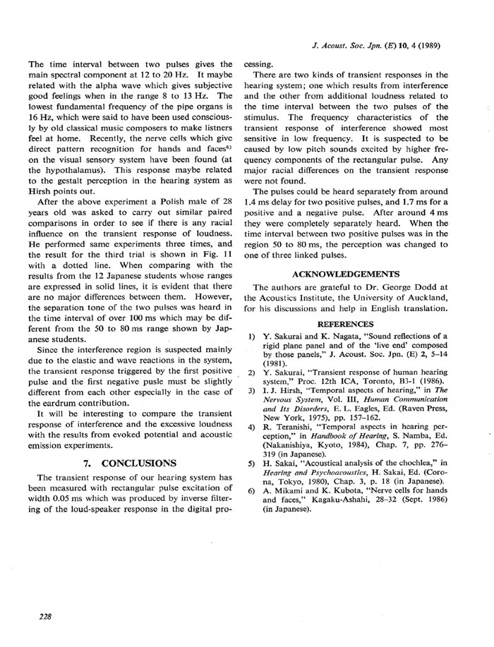
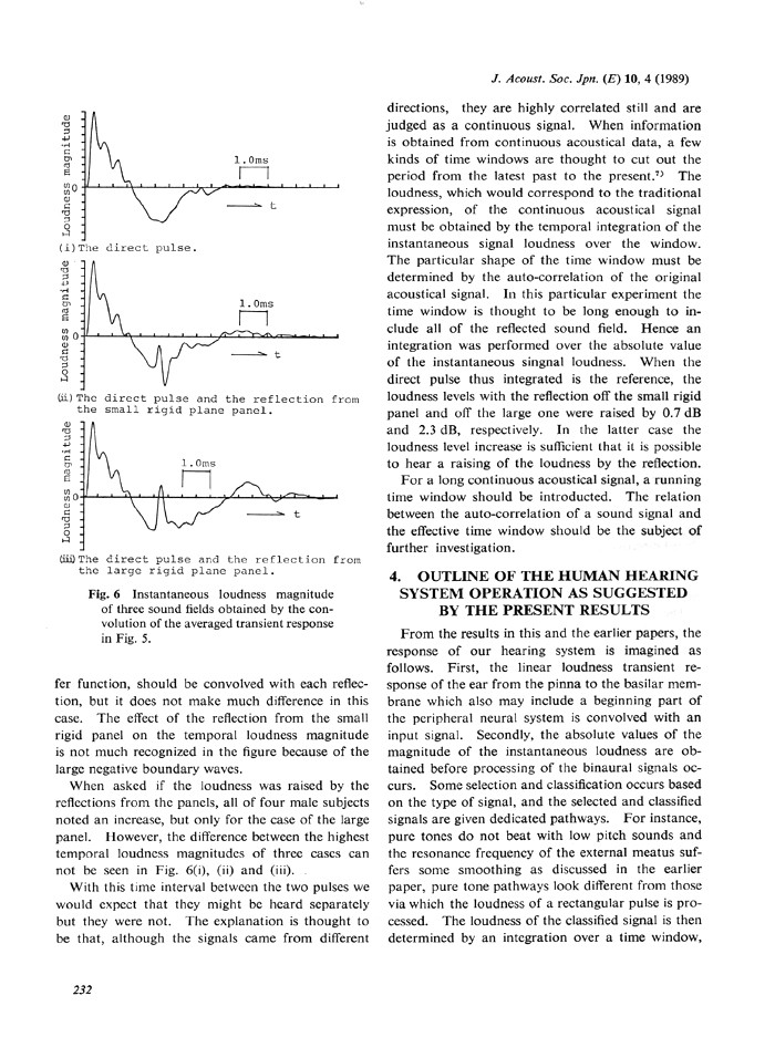
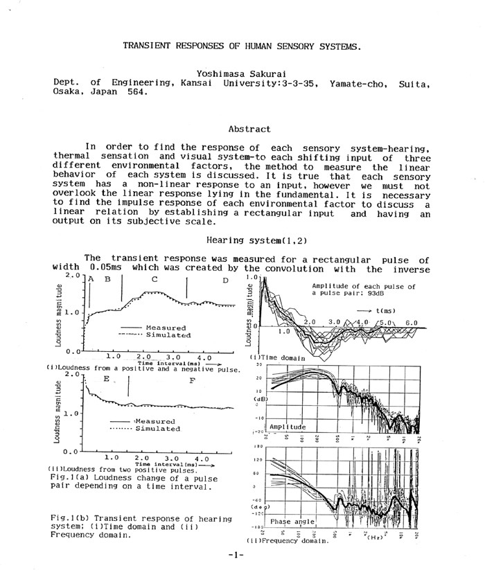
H-1-1) Impulse response of our hearing system R (t)
Measurement of the transient response of the hearing system R (t) to a
0.05ms rectangular pulse was done. First, the rectangular pulse was
made with the inverse filter to the loud speaker. The added loudness of
two rectangular pulses with a time interval was compared with the
loudness of a single pulse to find their loudness. The impulse response
of the hearing system R (t) was obtained as in Fig.15.
Fig.15 Impulse response
of hearing system R (t)
Y. Sakurai and H. Morimoto: “Transient Response of Human
Hearing System”, J.A.S.Jpn (E).10.4. P221-228(1989)
The following eight pages are from the above reference.
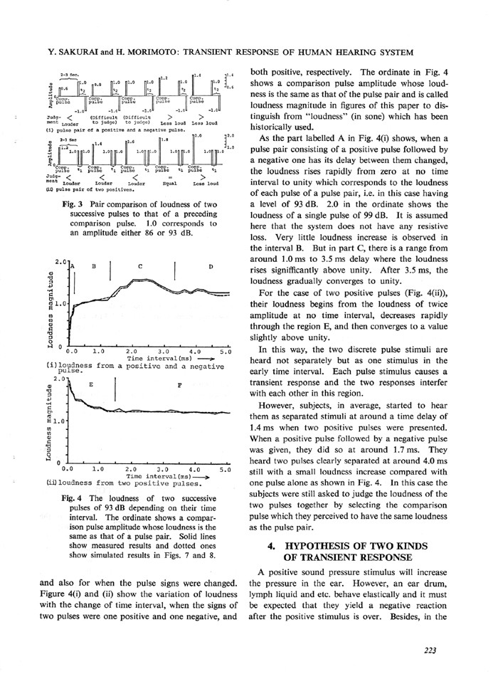
H-1-2) Absolutizing in our hearing system
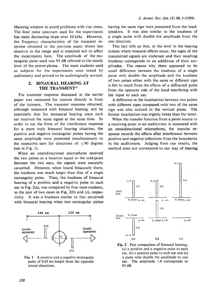
A positive rectangular pulse of 0.05ms width was given to one ear and a
negative one to the other ear as shown in Fig. 16. When a microphone
was at the head position the sounds were canceled. However, they were
heard as the loudness of two positive pulses. Our hearing system makes
a given signal to be absolutized after the linear response process.
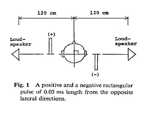
Fig.16 Certification of absolutizing processing
Reference; Y. Sakurai and H. Morimoto : “Binaural Hearing and
Time Window in the Transient”, J.A.S.Jpn(E) 10,4,
p229-233(1989)
The further explanation is given in the next five pages which are from
the above reference.
H-1-3) Loudness processing for a sound
A broad band noise and a pure tone are registered differently in the
brain for loudness processing, and the loudness for a sound of broad
band is thought to be decided:
(i) The sound is convolved with the impulse response of hearing system
R (t),
(ii) Its absolute value is obtained before it reaches the binaural
processing
(iii) During this process, the signal is classified and takes its
pathway
The low pitch sound of two pure tones does not beat with a pure tone
given from outside and the resonances at the outer ear are smoothed in
the impulse response for a broad band noise, a pure tone and a broad
band sound go through different ways to be registered.
(iv) A time window, which might be different with a kind of a sound
(its information) and its time pattern (autocorrelation function), is
given, and,
(iv) Its result is integrated in the time window.
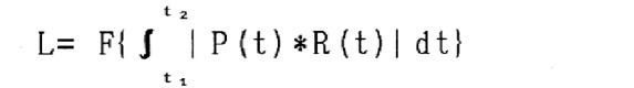
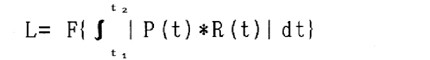
It is expressed,
where t1~t2 is the time
window and 40ms is for a noise[1]. P (t) is a
sound pressure, and R (t) is an impulse response of the hearing system.
* shows a convolution product. A function F could be a power or a
logarithmic function. The non-linear filter of logarithm or power is
made by the saturation of excessive input in the high level and by the
inner noise of biological activities, and the loudness of the sound is
given.
[1] Y. Sakurai et al:”Loudness of a given impact
sound”,
p209-212, Kinki Branch Meeting of the A.I.J. (1990) ( in Japanese
language ).
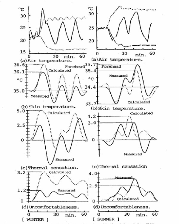
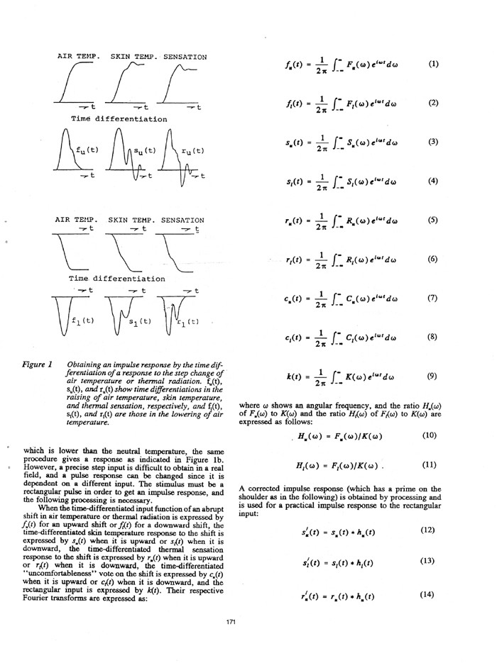
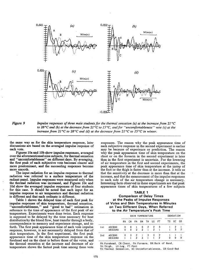
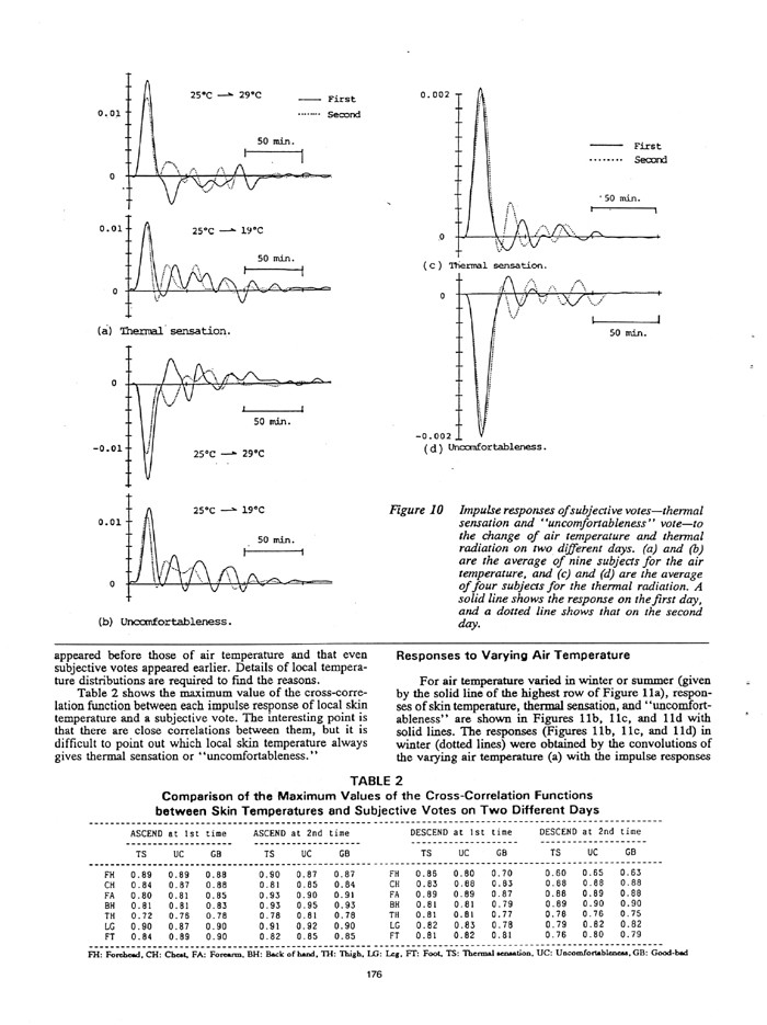
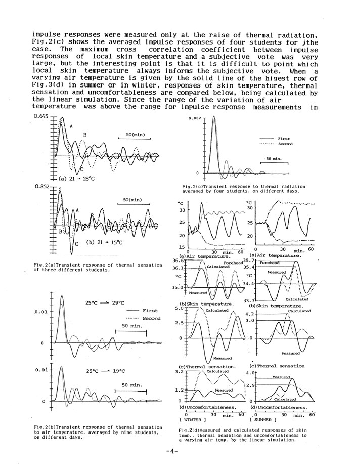
H-2) Thermal sensations
Thermal sensation was obtained every minute when a step function change
was given to each side from the neutral temperature. It is shown at the
air temperature change in Fig. 17. The response was differentiated to
get the impulse response for thermal sensation. The neutral temperature
was different in summer and winter. The impulse responses for skin
temperature were also measured. They are given in Fig. 10 (see the
reference below).
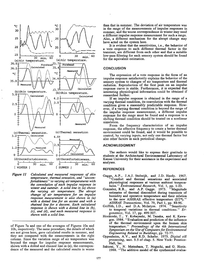
Fig.17 Comparison of
measured and calculated results for skin temperature and thermal
sensation for fluctuating temperature.
For a fluctuating temperature change it was convolved with the impulse
response and the result was compared with a practical thermal sensation
as shown in Fig.17.
The impulse response was obtained with the magnitude estimation, and it
must be carefully used in the measured range.
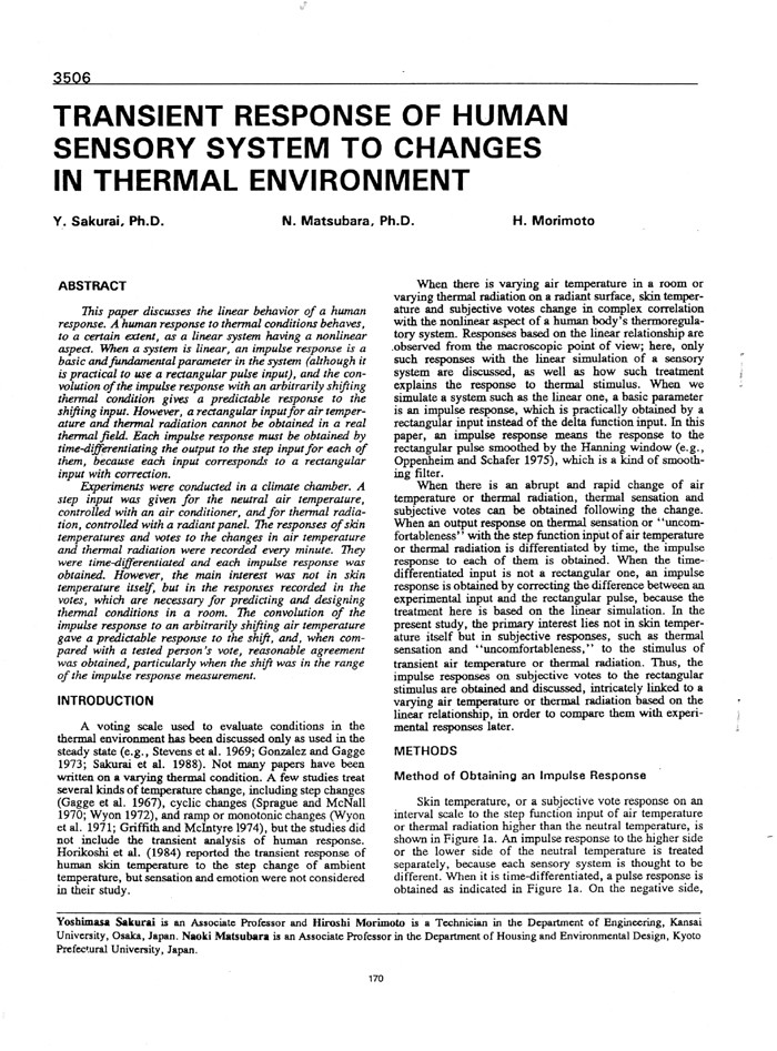
Reference ; Y. Sakurai et al: “Transient Response of Human
Sensory System to Changes in Thermal Environment”, ASHRAE
(3506),-p170-178,
The next 9 pages are from the above reference.
*******************************************************************************************
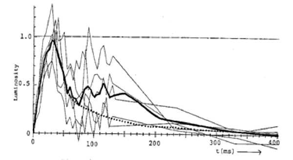
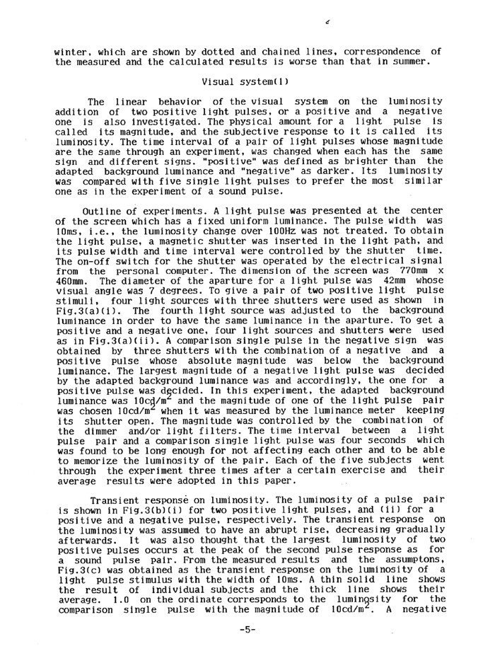
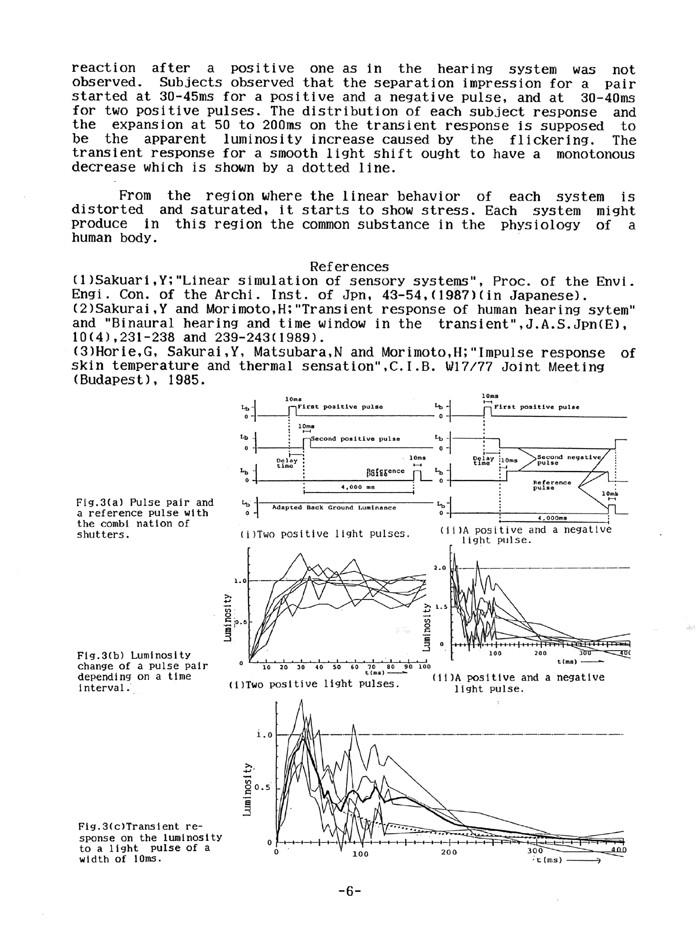
H-3) Impulse response for brightness
An aperture was given in the middle of a large uniformly illuminated
panel for adaptation brightness. At the aperture a brighter or a darker
light pulse was given with a certain time interval and their
interference was measured.
Fig.18 Brightness impulse
response for a light pulse
It is supposed that the deviation from 60 to 120 ms was caused by the
flickering of the light source. The response in this region and later
was smoothed by eliminating the deviation as shown by a dotted curve in
Fig. 18.
Reference; Y. Sakurai and T. Noguchi:"Transient response of the human
visual system to a light pulse", p157-158, Oct. 1989, Archi. Inst. of
Jpn (Kyushu) ( in Japanese language ).
More explanation is given in the next two pages from the reference [1]
in the next section.
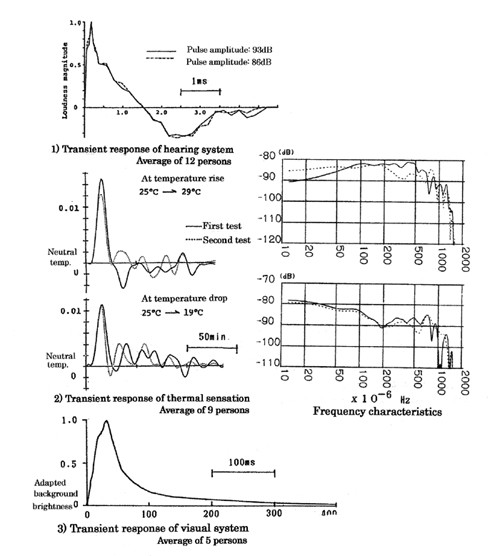
H-4) Summaries of impulse responses for three sensory systems
Impulse responses for three different sensation systems are summarized
in the next figure.
We have to keep discussing each sensation processing in relation to
each other one.
Each sensory system’s impulse response is compared as above
and it is interestingly different.
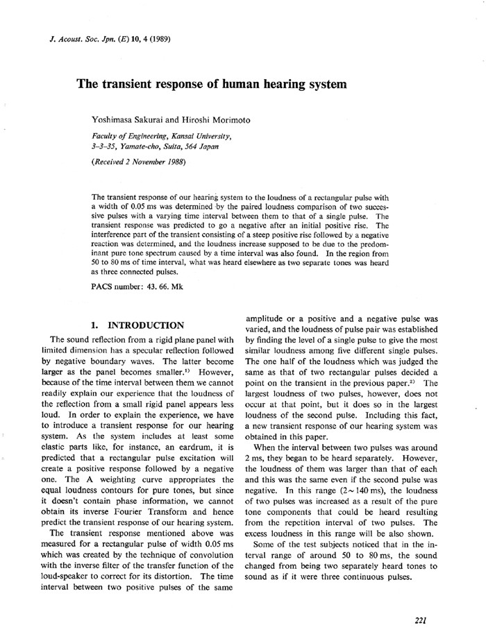
In the hearing system, after an abrupt rise, it gradually decreases and
then shows a negative response. It must be caused by the elastic
reaction of the ear drum, the little bones, the basilar membrane and
the lymph liquid in the cochlea. When one of the trial volunteers
listened to a 50msec rectangular pulse, he got the impression of
hearing a higher frequency component earlier and lower one later. The
former impression was given by the front part of the basilar membrane
and the latter one was from the rear part.
When the experiments were done with the rectangular pulse of 7dB lower,
we got the same response. It means that the impulse response was
obtained as the linear response of the auditory system, I mention it
again here.
In the end, at the stage when each system proceeds to saturation after
the linear process, it is supposed that one starts to get stressed and
the resulting energy must be released somewhere. Every system is
supposed to yield such substance commonly which is caused by the stress
and the one which resists the stress. We should discuss how we could
use them as indicators to be stressed or not, and realize stress free
circumstances.
It is true that each sensory system has a non-linear response but we
must not overlook its linear response in the earlier stage. For that, a
rectangular input for each factor must be well defined, and we can find
its response.
Reference: Y. Sakurai: “Transient Responses of Human Sensory
Systems”,
Material at a symposium for “Physiological and psychological
dynamics for Architectural environmental design” p2
– 18,
30/11/1990, Nagoya (in Japanese).
[1] Y. Sakurai:”Transient Responses of Human
Sensory Systems", p21-24、Oct., 1989, Psycho-physics (Cassis, France)
The following six pages are from the above reference [1].
Some
additional comments on specific and combined ratings
If circumstances are comfortable, we do not mention it all the time and
it always changes. It is difficult to find the relation between a
physical input and the output that is not always observable. On the
other hand, an environment of discomfort is immediately perceived and
expressed, and it is easier to find the relation in between. It is a
technical matter to improve the environment to eliminate the discomfort.
Besides, the uncomfortableness of each heterogeneous factor is additive
and a multi-variable indoor environment was quantified applying the
theory of quantification II as shown in the section C). Now, we can
discuss each factor on the common scores for environmental planning.
The technical and financial difficulties can be compared on the same
basis.
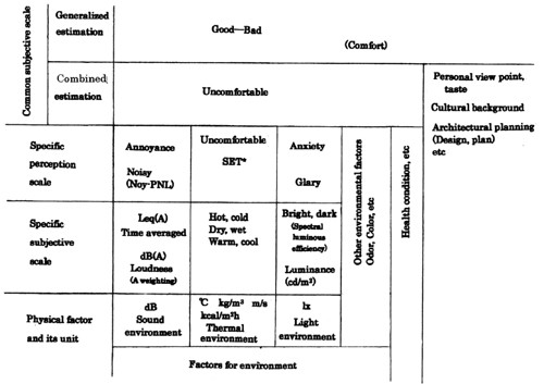
There exist a variety of subjective scales on a daily life, e.g.
specific subjective scales, combined subjective scale, generalized
scale etc. the following table is an overview of them.
When we look at it, specific perceived scale to rate a light
environment is not fully introduced yet. We need a scale to have
spacious rating at a practical situation.
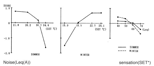
An idea to find the relationship between the steady state combined
rating and combined rating for a changing environment
Uncomfortableness scores for sound and thermal environments are
expressed on the vertical axis with a specific physical scale for each
factor on the horizontal axis in the next figure.
Uncomfortableness score
vs specific physical scale
The specific physical scales for the loudness of a noise and thermal
sensation are supposed to be simulated the specific subjective scales
and they change linearly or smoothly on their physical scales, but
these curves have points of inflection. It is interesting that the
uncomfortableness suddenly increases from there.
It shows actually a functional expression for uncomfortableness towards
physical parameters. In this way, we can find the relationship between
the uncomfortableness scale and specific subjective scale for an
environmental factor through its physical simulation.
How could it be connected to scores for a changing environment? When we
look back at a sound environment, sound pressure was contracted to a
logarithmic scale because of its wide audible range to a dB scale. It
simulates our hearing system with the “A “
weighting. For a
changeable noise its time average is obtained to give Leq (A).
As I mentioned at the section for the loudness of an impact noise, I
estimated as follows.
Loudness processing for a broad band noise and a pure tone are
registered differently in the brain, and the loudness for a sound of
broad band is thought to be decided by:
(i) The sound is convolved with the impulse response of hearing system
R (t),
(ii) Its absolute value is obtained before it reaches the binaural
processing,
(iii) During these process, the signal is classified and takes its
pathway,
The low pitch sound of two pure tones does not beat with a pure tone
given from outside and the resonances at the outer ear are smoothed in
the impulse response for a broad band noise, a pure tone and a broad
band sound go through different pathways to be registered.
(iv) A time window, which might be different with a kind of a sound
(its information) and its time pattern (autocorrelation function), is
given, and,
(iv) Its result is integrated in the time window.
It is expressed,
where t1~t2 is the time
window and 40ms is for an impact noise[1]. P
(t) i s sound pressure, and R (t) is an impulse response of the hearing
system. * shows a convolution product. A function F could be a power or
a logarithmic function. The non-linear filter of logarithm or power is
made by the saturation of excessive input in the high level and by the
inner noise of biological activities, and the loudness of the sound is
perceived.
The discussion was on an impact sound and did not apply to usual noise,
like street traffic noise. However, when the methodology is applied on
it and find its specific physical scale, it could be compared with the
uncomfortableness scale.
This kind of discussion on noise rating can be done for two other
factors. Their impulse responses are already obtained as shown, the
similar items, for instance, a time window, non-linear processing, must
be introduced how their specific physical scale simulate their
sensitivities.
When the impulse response of thermal sensation was obtained, the
response included the magnitude estimation and further discussion is
necessary.
In such a way, the uncomfortableness scale as a combined rating is
introduced, being related to each specific scale, we could support
sustainable living.
Though comfort is subjective, we have to discuss the background to how
it happens. What we should study is what is conditioned for a man, and
what his biological nature is. There is a range where two successive
rectangular pulses are heard as if three pulses are given. This kind of
responses, such as Gestalt recognition of a face or of a hand is
another example,
When we often enjoy good music, the enjoyment is caused by the
conditioned response.
It is important to find such physical factors to have such results and
apply them to create a better space and time.
If we are conditioned by accumulated past experiences, such as a
defensive or protective response to a sudden large impact sound, it is
not included in the combined rating. It must be added as an independent
factor. Such sudden impact happens not only for sound, but for
vibration, light, temperature change etc.
Related discussion has been done mainly on the time domain, but we have
to discuss it for space as well. For instance, in a sound field we
quite accurately discern direction as is shown in Chap 6. How it should
be combined with the response in the time domain must be discussed.
I) Combination of two sensory systems; vision and hearing
Contradiction of an acoustics theory of localization for a sound source
is described here, when it is related with vision.
When I was watching a movie in front of a large screen, I felt the
sound was coming from there but the stereo audio system was behind me.
This has a contradiction of the sound source localization with the
first wave front.
With a smaller screen, the location of the sound source and the visual
image were not in the same direction, and the sound impression was
moved to lateral front instead of having the real location behind.
And the sound image remained there even after the screen was off. That
shows it to be a learnt impression.
Mutual interactions between sensations must be further studied, as well
as each one.
Reference: G. Dodd and Y. Sakurai, “Localization of sound
– a New
Zealand Revelation”, New Zealand Acoustics, p28-33, No4,
Vol16
(Dec, 2003)
Following pages are from the above reference.
The above interesting observation was a recent one. It tells us that
each sensation can not be independent. It can easily be imagined
through experiences that a specific subjective scale is affected by
other environmental factors. For instance, we tend to feel an
environment noisier when it is very hot or hotter when it is very
noisy. It would be interesting to find how it interacts on the
uncomfortableness subjective scale.
This chapter has written as a guide line to plan for a comfortable
living environment, using the combined rating. However, it is just a
technological help to avoid an uncomfortable environment. We do not
need to mention that each one has to add to it with own expression and
creation.
For planning sustainable living, the first issue of house designing is
to use solar energy in the best way. There we need to find the living
condition not qualitatively but quantitatively.
It may be an idea for a model house to show how much of energy
consumption cost for heating could be saved, depending on a plan of the
house at the actual local site.
We need a good computer program to predict it and have to urgently
educate young people to handle it properly. We need well trained
consultants for the community.
The theories of quantification by Hayashi are very useful tools for a
multi-variable field. The method can be useful also for medical
purposes, agriculture etc. Sickness does not have only one cause, and
crops grow differently depending on a variety of factors such as
geographical and geological conditions.
If one starts to establish a sustainable way of living at younger age,
it can be achieved more easily. It can be said too for learning
technology and science.
It is not difficult to live sustainable relying only on solar energy
and it is the only way to establish one’s freedom and
creative
world.
If one starts a new subject without any fear or concern, anything comes
out and be created. With the creation, further progress can be
expected. Instead of seeking progress only in one’s thought,
to
do it in realty is a better result, I think.